Blog written by Sean Roberts, Research Associate, Anthropology and Archaeology, University of Bristol

Causal graphs

Causal graphs are great ways of expressing your idea about how the world works. They can also help you design your analyses, including choosing what you need to control for in order to exclude alternative explanations for the patterns you find. Standard methods about how to choose control variables are often vague (Pearl & Mackenzie, 2018), and many assume that controlling for more variables makes the central test more robust. However, controlling for some variables can create spurious correlations due to colliders. This is very worrying! But if we draw our ideas as causal graphs, then we can spot colliders and try to avoid them.

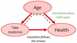
Pearl & Mackenzie (2018) talk about causality and correlation in terms of the flow of information. Causal effects ‘flow’ between nodes following the causal arrows, but correlation can flow both ways. In the example below, taking a certain medicine might affect your health. But your age might affect both your health and whether you remember to take the medicine. In this case, there might be a correlation between taking medicine and health either because of the causal connection (the causal path), or because of the confounding correlational path though age (the non-causal path):

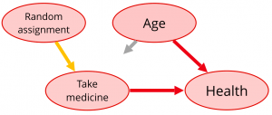
In a randomised control experiment, the link between health and taking medicine might be blocked by intervening and randomly assigning who takes the medicine (and in this hypothetical example, ensuring that they do take the medicine). That is, the only thing that decides whether the medicine is taken is our experimenter’s random decision. This means that the only path which connects medicine and health (in our hypothesis) is the causal path that we are interested in.

Blocking causal paths can also be done by ‘conditioning’, for example controlling for the effect of age in a statistical regression:

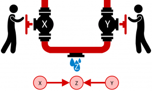
The final thing that can block a correlation path is a collider. A collider is a node on a causal path with two causal links (arrows) pointing into it. In the graph below, X and Y affect Z. We wouldn’t expect a correlation between X and Y, because that path is blocked by the collider at Z.

Colliders behave differently to other causal structures. Below are the four different types of connection between three nodes (excluding ones where X and Y are connected). In the first three, there is a path between X and Y, so X and Y should be correlated. This is the root of one of the central problems in research: we cannot tell the first three systems apart just by observation. We would have to manipulate one of the variables (e.g. in an intervention study) and see whether it had an effect.

In the first two graphs, Z is a ‘pipe’. It connects X and Y. If we were to intervene or control for Z, then the relationship between X and Y would be broken and there should be no correlation. In a statistical framework, we would not want to control for Z. The third system, X and Y are correlated due to a ‘common cause’ or ‘fork’ in Z. However, the behaviour is the same: X and Y should be correlated except for when we control for Z.

The final example is a ‘collider’, and it is different from the rest. Here, X and Y are not correlated except for when we control for Z, at which point they will become correlated (Elwert 2013).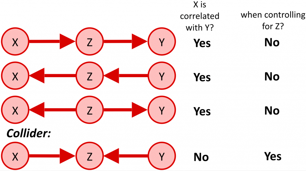

To help understand this, imagine that you and I are working at a waterworks. We can each control the rate of flow in our pipe (X and Y) and our pipes are connected so that the final rate of flow is the combined rate from each of us, Z. I can turn my cog independently of you, and vice versa.

If you turn your rate up it increases the flow in Z, but that has no effect on me, so our rates (X and Y) should not be correlated. However, then our manager calls and tells us that we have to maintain a certain rate of flow in Z (they are conditioning or fixing Z). Now, if I turn my rate up, then you have to turn your rate down to maintain the required rate in Z. And if you turn your rate down, I have to turn my rate up. So someone observing X and Y would see a correlation. That is, X and Y are not correlated, except for when conditioning on Z.

So, correlations will be blocked by a collider unless we control for it, at which point the correlation path ‘opens up’ again.

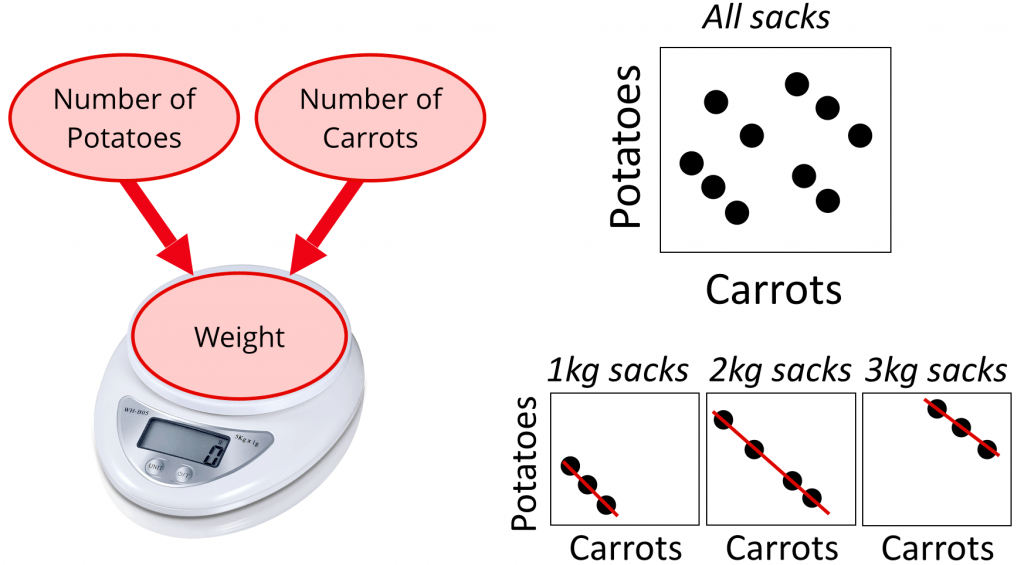
Here’s another example. Imagine we’re filling sacks with potatoes and carrots. The weight depends independently on each vegetable, and there’s no correlation between them. But if we split the observations by weight, then the number of potatoes predicts the number of carrots.

The behaviour of colliders means that controlling for some variables can lead to spurious correlations (Elwert & Winship 2014, Ding & Miratrix 2015, Westfall & Yarkoni 2016, Rohrer 2018, Middleton et al 2016, York 2018).

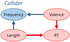
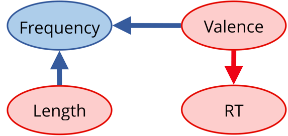
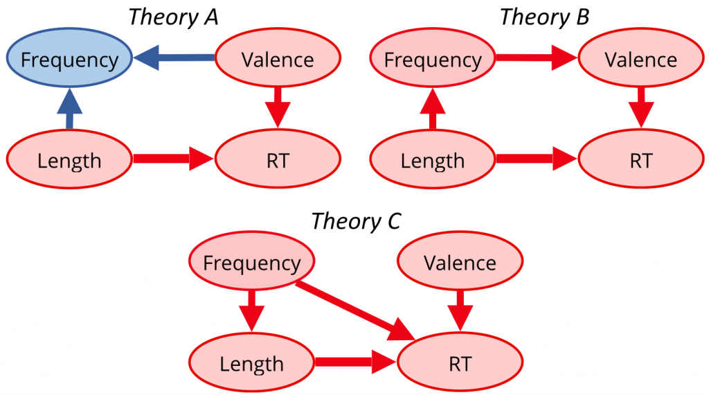
Considering colliders is important when deciding which variables to control for in a statistical test. Imagine that we’re investigating reaction times (RT) in reading, and we have measured the length of a word, reaction times for reading the word, the frequency of the word and the word’s valence (the degree of pleasantness of the meaning of the word). We’re interested in testing whether word length affects reaction time. What should we control for? Let’s say that we have the following hypotheses: frequency is affected by length (Zipf’s law, Zipf 1935) and valence (Polyanna hypothesis, Boucher & Osgood 1969), and valence affects reaction time (e.g. Kuperman, Stadthagen-Gonzalez & Brysbaert 2012):

Frequency is actually a collider along the path from length to valence. This means that, although there is a non-causal path between length and RT, the flow of information is blocked. In this case, we should not control for frequency in our statistical model, since doing so would cause length and valence to become correlated, opening up a non-causal path from length to RT.

This is not a hypothetical problem. It will genuinely affect real analyses. For example, in the R code below, we create some artificial data generated by a world where there is no causal path between length and RT:

<code>

n = 200

length =  sample(1:7, n, replace = T)

valence = sample(1:7, n, replace = T)

freq = length + valence + rnorm(n)

RT = valence + rnorm(n)

</code>

We can run a statistical model, predicting reaction time by length and we see that there is no significant correlation (as we expected):

<code>

summary(lm(RT ~ length))

Estimate Std. Error t value Pr(>|t|)

length      -0.03436    0.07971  -0.431    0.667

</code>

However, when we add frequency as an independent variable, suddenly both length and frequency are significantly correlated with RT:

<code>

summary(lm(RT ~ length + freq))

Estimate Std. Error t value Pr(>|t|)

length      -0.83004    0.06520 -12.730   <0.001 ***

freq         0.85081    0.04647  18.310   <0.001 ***

</code>

Of course, this may not be the correct or complete causal model in the real world. There are many possible models (some of them don’t have colliders and so you should control for frequency). The point is that your hypothesis should affect the design of your statistical model or your experimental manipulations. Throwing all your variables into the model may actually worsen your ability to infer what’s happening.

It is therefore vital to clearly define our prior hypotheses, and causal graphs are an excellent way of doing this.

As Pearl & Mackenzie explain, we can use causal graphs to identify variables that we should control for. If we’re interested in the effect of X on Y, then we might be able to calculate:

The observational relationship between X and Y (e.g. probability of observing Y given X).
The state of Y if we were to manipulate X (an intervention)

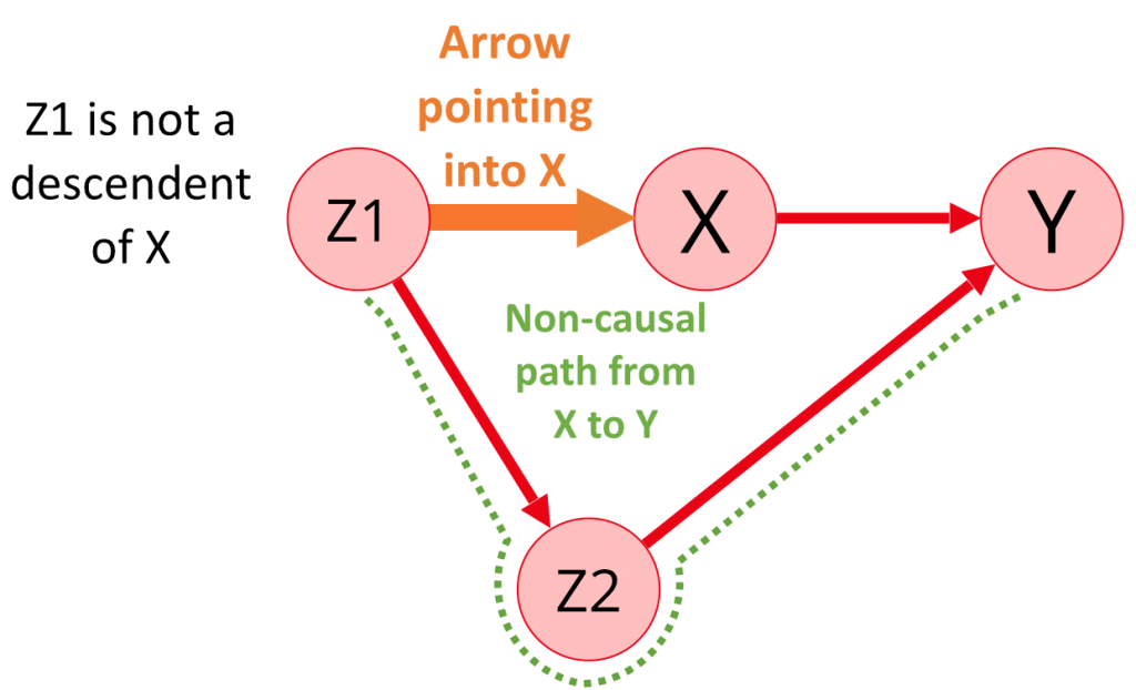
A confounding variable is anything that leads to a difference between these two calculations. To remove confounding, we need to block every non-causal path without blocking any causal paths (block any ‘back door paths’). This means we should control for any variable Z on a non-causal path from X to Y that starts with an arrow pointing to X and where Z is not a descendant of X (there’s no way to get from X to the Z following causal paths, see Shrier & Platt 2008).

In the example below, there is a path from X to Y through Z1 and Z2, so we should control for either Z1 or Z2 (or both) in order to block this non-causal path.

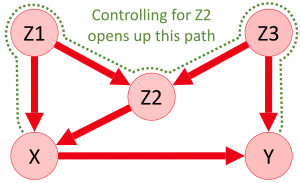
Other examples can become more complicated. For example, in the graph below, there is a non-causal path that needs to be closed: X – Z2 – Z3 – Y. However, controlling for Z2 creates a correlation between Z1 and Z3, opening a new non-causal path. In this case we should control for Z3 rather than Z2.

Tools like Dagitty have algorithms for calculating the options for which variables should be controlled for. The Causal Hypotheses in Evolutionary Linguistics Database (CHIELD is a database of causal claims with tools for exploring connections between them. Graphs in CHIELD can be exported to Dagitty.

A causal approach to research asks us to be brave and make commitments about how we think the world works. If we do this, we might be able to make better decisions and to extract a lot more from our data than we expected.

CHIELD

CHIELD is a searchable database of causal hypotheses in evolutionary linguistics. It has tools for expressing and exploring hypotheses. Anyone can contribute, and the code is open source for other fields to build their own databases. Contact sean.roberts@bristol.ac.uk for more information.

A brief introduction to colliders

Blog written by Sean Roberts, Research Associate, Anthropology and Archaeology, University of Bristol

Causal graphs

CHIELD

Recommended reading