Blog written by Rob Arbon, Data Scientist at the University of Bristol.

This project was funded by the annual Jean Golding Institute seed corn funding scheme.

Multitask learning for AMR

“Multitask learning for AMR” developed out of our collaboration with the Jean Golding Institute on the One Health Selection and Transmission of Antimicrobial Resistance (OH-STAR) project funded by the Natural Environment Research Council (NERC), the Biotechnology and Biological Sciences Research Council (BBSRC) and the Medical Research Council (MRC).

OH-STAR is seeking to understand how human activity and interactions between the environment, animals and people lead to the selection and transmission of Antimicrobial Resistance (AMR) within and between these three sectors. As part of this project we collected thousands of observations, from over 50 dairy farms, of the prevalence of AMR bacteria, as well over 300 potential environmental variables and farm management practices which could lead to AMR transmission or selection (so called risk factors). If we can identify these risk factors the hope is that we can use this information to shape policy to reduce the spread of AMR into the human population where it threatens to cause widespread death and disease.

Multitask learning (MTL) is a statistical technique that aims to relate different “tasks” in order to improve how we perform those tasks separately and to understand how the tasks are related. MTL has been used in many different areas from improving image recognition and to help diagnose neurodegenerative diseases. In this project we wanted to see if MTL could be used to help better understand the OH-STAR data and also to sketch out ideas for potential grant applications to develop this idea further.

To evaluate MTL for our purposes, we focused our attention on two small subsets of the OH-STAR data: 600 faecal samples from pre-weaned young calves and 1800 from adult dairy cows. Each of these samples had been tested to see whether the Escherichia coli. bacteria within them contained the CTX-M  gene. This gene is important because it confers resistance to a range of antibiotics such as penicillin-like  and cephalosporin antibiotics which are used to treat a range of different infections  in humans and cattle.

In order to model the risk of something occurring, statisticians use a technique called logistic regression. With this technique you can quantify by how much a risk factor, e.g. which antibiotics a farmer may use,  increases or decreases the risk of observing the CTX-M gene in samples from the farm. As an example, consider how one of our risk factors, atmospheric temperature, affects the risk of observing CTX-M. Each dot on the chart below represents one of our samples, whether it had CTX-M (right hand axis), and the temperature when the sample was recorded (horizontal axis). The results of the logistic regression are the black line (left hand axis): the risk of observing CTX-M as the temperature increases.

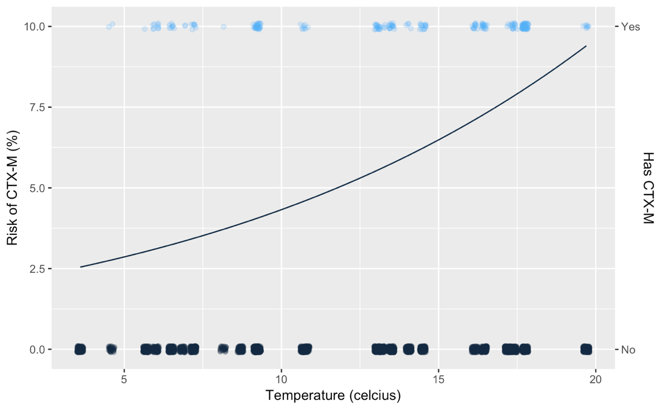
This relationship can be summarised by a single number called the log-odds-ratio, in this case the log-odds-ratio of temperature is 0.4. The fact that this number is greater than 0 means the temperature increases the risk of CTX-M, if it were less zero this means that it decreases the risk.

So, to quantify how each of the measured risk factors affects the risk of observing CTX-M we could just use logistic regression on all 300 risk factors for both the adults and separately for the calves  and look at the log-odds-ratios for each risk factor. This approach suffers from two problems however:

1. by fitting a standard logistic regression model with 300 risk factors and at most 1800 observations means your conclusions won’t necessarily be correct for a wider population (because of overfitting)
2. this approach treats understanding risk in adults and heifers as two separate tasks, when in fact they share many similarities.

To overcome the first problem statisticians use a technique called regularization. In a nutshell this reduces the complexity of your model to prevent it predicting random points (“noise”) in your data and focuses the model on predicting the “true” signal.

Multi-task learning (MTL) is an approach to overcoming the second problem. The idea is that some risk factors will pertain more to calves than to adults (e.g. the type of antibiotics given when they are young) or vice versa. So it makes sense for these risk factors to have different impacts on the model. However, there are some risk factors that will have very similar effects on both types of animal (e.g. outside temperature ). The way MTL relates tasks is complicated but it is very similar to the regularization technique linked to above. Interested readers can read reviews of MTL in A brief review on multi-task learning and An overview of multi-task learning in deep neural networks.

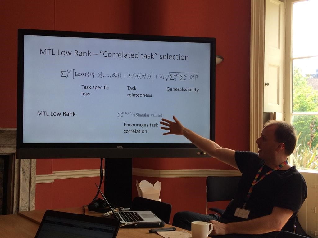
We looked at a number of different MTL techniques using the R package RMTL (package and accompanying paper) but for brevity we will consider only one here. Our two ‘tasks’ were logistic regression to find the risk factors affecting pre-weaned calves (task 1, labelled ‘heifers’) and adults (task 2).

The technique I’d like to talk about here is called ‘Joint feature learning’ and relates the tasks by encouraging them to have similar values for each risk factor. This means that if they’re not important for both, they will feature less strongly in each model. The results are shown below for the results with (right) and without (left) MTL.

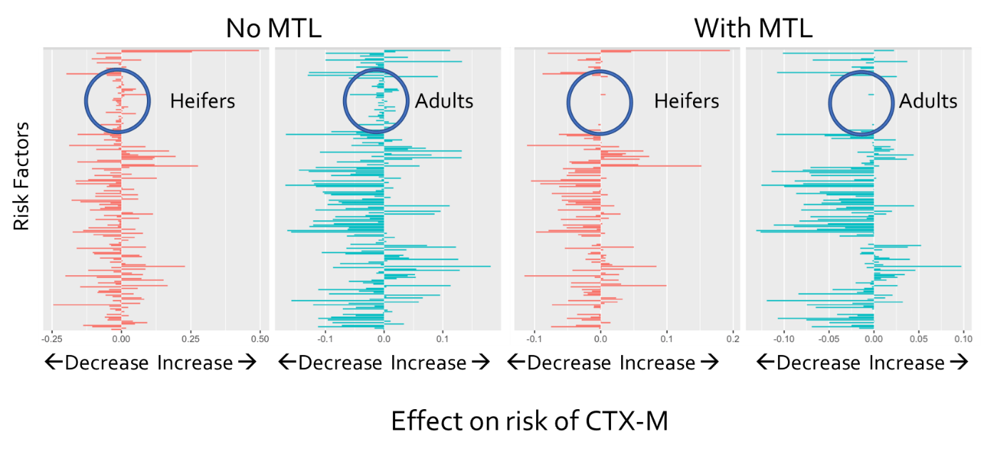
The red results are for heifers and the blue results are for the adults. Each bar denotes the effect of a risk factor on the risk of observing CTX-M: positive increases the risk while negative decreases the risk. The effect of using MTL was to suggest that the circled risk factors were not important to both tasks as applying MTL made all those risk factors irrelevant to the task. This was important for two reasons.

First, this cut down on the number  of possible risk factors that needed further investigation. Second, this meant that those risk factors which did show up as having different effects on the risk could be trusted as not being down to just chance. For example, temperature was one of the most important features for the heifers but not for the adults – this could provide ideas for interesting hypotheses to test in future work.

MTL has potential novel applications in real world scenarios

The main conclusion from this work is that MTL has potentially novel applications in complicated “real-world” scenarios but that the tools for MTL need developing. For example the techniques in the RMTL package did not fully take into account the structure of the data. This is something that will need to be addressed in any future work.

In our wrap up meeting we discussed the potential for using these techniques in future work. The main idea discussed was to use data collected as part of a completely separate project to help understand risk in OH-STAR data and vice versa. For example, the One Health drivers of AMR in rural Thailand (OH-DART) is a similar project, funded by the Global Challenges Relief Fund (GCRF). The distinct but related datasets from OH-STAR and OH-DART projects could be analysed jointly using MTL to identify risk factors. Thanks to the funding from the JGI we now have the materials necessary to write such a proposal and we will be watching calls from e.g. the GCRF and BBSRC in the near future to fund this work.

All of our code for this work can be found on the Open Science Framework.

The Jean Golding Institute seed corn funding scheme

The JGI offer funding to a handful of small pilot projects every year in our seed corn funding scheme – our next round of funding will be launched in the Autumn of 2019. Find out more about the funding and the projects we have supported.

 

 

Blog written by Dr Stephen Chuter, Research Associate in Sea Level Research, School of Geographical Sciences, University of Bristol

This project was funded by the annual Jean Golding Institute seed corn funding scheme.

Antarctica and sea level – a grand socioeconomic challenge

Global sea level rise is one of the most pressing societal and economic challenges we face today. A rise of over 2 m by 2100 cannot be discounted (Ice sheet contributions to future sea-level rise from structured expert judgement), potentially displacing 187 million people from low-lying coastal communities. As a major and increasing contributor to global sea level rise, it is of critical importance to understand and quantify trends in the mass of the Antarctic Ice Sheet. Additionally, effective communication of this information is vital for policy makers, researchers and the wider public.

Combining diverse observations requires new statistical approaches

The Antarctic Ice Sheet is larger in area than the contiguous United States, meaning the only way to get a complete picture of its change through time is by using satellite and/or airborne remote sensing to supplement relatively sparse field observations. Combining these datasets is a key computational and statistical challenge due to the large data volumes and the vastly different spatial and temporal resolutions of different techniques. This challenge, which continues to grow as the length of the observation record increases and as new remote sensing technologies provide ever higher resolution data, requires new and novel statistical approaches.

We previously developed a Bayesian hierarchical modelling approach as part of the NERC-funded RATES project, which combined diverse observations in a statistically-rigorous manner. It allowed us to calculate the total mass trend at an individual drainage basin scale, in addition to the relative contribution of the individual component processes driving this change; such as variations in ice flow or snowfall. Being able to study the spatial and temporal pattern of the component process allows researchers to better understand what the key external drivers of ice sheet change are, which becomes critical when making predictions regarding about its future evolution.

Project goals

Our current work is aiming to achieve two major goals:

1. Develop the Bayesian hierarchical framework and incorporate the latest observations in order to extend the mass trend time series until as close as possible to the present day.
2. Synthesise the results in an easily accessible web application, so that users can interrogate and visualise the results at a variety of spatial scales.

The first of these goals is critical to providing model and dataset improvements, paving the way for the framework to be used over longer time series in order to better understand multi-decadal processes. The second goal, funded by the JGI seed corn award, is to provide these outputs in a manner that is easily used and understood by a range of stakeholders:

• Scientists – Ability to use the latest available results within their own research and as part of large international collaborative inter-comparisons (e.g. World Climate Research Programme).
• Policy makers – Allows easy interrogation of the results and have an accessible overview of the methodology. This will allow for project outputs to be easier included as evidence in policy making decisions.
• General public – Generate public interest in the research output, the method used and raise awareness of the potential impacts of climate change on ice sheet dynamics.

Results

To date we have extended mass trends for the Antarctic Ice Sheet up to and including 2015. This has enabled us to see the onset of dynamic thinning (changes in mass due to increased ice flow into the ocean) over areas previously considered stable such as the Bellingshausen Sea Sector and glaciers flowing into the Getz Ice Shelf.

The cyan line represents total ice sheet mass change, the orange line represents changes due to ice dynamics (variations in ice flow) and the purple line represents changes in mass due to surface processes (variations in mass due to changes in precipitation and surface melt). The shaded areas around each line represent the one standard deviation uncertainty.  

In order to disseminate these results, a new web application has been developed. This allows users to interactively explore and download the updated results. Additionally, the web application features a second interactive page, aimed at the public and policy makers, which provides an overview of the datasets used in this work.  

Future plans

The project has allowed us to make key advances in this methodology, laying the foundations for extending the time series nearer to the present day. Future plans include incorporating additional observations from the new ICESat-2 and GRACE follow-on satellite missions. Ultimately, the extended time series will be an important input dataset for the GlobalMass ERC project, which aims to take the same statistical approach to study the global sea level budget.  

The creation of the web application will allow for future updates to be quickly communicated, which allows our results to be incorporated in related research or policy making decisions. We hope to extend the web application functionality further to include more outputs from the GlobalMass project. 

The Jean Golding Institute seed corn funding scheme

The JGI offer funding to a handful of small pilot projects every year in our seed corn funding scheme – our next round of funding will be launched in the Autumn of 2019. Find out more about the funding and the projects we have supported.

Blog written by Jonty Rougier, Professor of Statistical Science.

Data are a precious resource, but easily corrupted through avoidable poor practices. This blog outlines a lightweight approach for ensuring a high level of integrity for datasets held as computer files and used by several people. There are more hi-tech approaches using a common repository and version control (e.g. https://github.com/), but they are more opaque.

If this approach is accompanied by this document (in the same folder) then there should be no loss of continuity if there are personnel changes. It might be helpful to create a file README stating: See *_safeguarding.pdf for details about how these files are managed.

The first point is the most important one:

1. Appoint someone as the Data Manager (DM). All requests for datasets are directed ‘upwards’ to the DM: do not share datasets ‘horizontally’. The DM may respond individually to dataset requests, or they may create an accessible folder containing the current versions of the datasets (see below).

The following points concern how the DM manages datasets:

2. Each dataset is a single file, with a name of the form DSNAME.xlsx (not necessarily an Excel spreadsheet, although this is a common format for storing datasets). At any time, there is a single current version of each dataset, with the name yyyymmdd_DSNAME.xlsx; the prefix yyyymmdd shows the date at which this file became the current version of DSNAME.xlsx. The current version is the one which is distributed. Everyone should identify their analysis according to the full name of the current version of the dataset. This makes it easier to reproduce old calculations, and to figure out why things work differently when the dataset is updated.

3. The DM never opens the current version. They simply distribute it (including to themself, if necessary). This is very important for spreadsheets, where every time the file is opened, there is the risk that entries in the cells will be inadvertently changed. Typically, though, new data will need to be added to DSNAME.xlsx, and corrections made. These changes are all passed upwards to the DM; they are not made on local versions of DSNAME.xlsx.

4. Incorporating changes. As well as current versions with different date prefixes, there will also be a development copy, named dev_DSNAME.xlsx. All changes occur in dev_DSNAME.xlsx. I recommend that each change to dev_DSNAME.xlsx is described by a sentence or two at the top of the file changes_DSNAME.txt. This file is made available alongside the current version of the dataset.

5. Updating the current version. When the changes in DSNAME.xlsx have become sufficient to distribute, it is copied to become the new current version, with an updated date prefix. The DM should alert the team that there is an update of DSNAME.xlsx. If the changes are being logged, insert the name of the new current version as a section heading at the top of changes_DSNAME.txt so that it is clear how the new current version differs from the old one.

6. If there is a crisis in DSNAME.xlsx then the DM should delete it, create a new dev file from the current version, and remake the changes. Crises happen from time to time, and it is a good idea not to accumulate too many changes in the dev file before creating a new current version. On the other hand, it can be tedious for people to be constantly updating their version for only minor changes. So the DM might want to create ‘backstop’ versions of the dev file for their own convenience, perhaps named backstop_DSNAME.xlsx, which also requires a line in changes_DSNAME.txt if it is being used.

7. The DM is responsible for backing up the entire folder. This folder contains, for each dataset: all of the current versions (with different date prefixes), the dev file, the changes file if it exists (recommended), and additional helpful files like a README. An obvious option is to locate the entire folder somewhere where there are automatic back-ups, but it is still the DM’s responsibility to know the back-up policy, and to monitor compliance; even to run a recovery exercise. It’s a bit ramshackle, but regularly creating a tar file of the folder and mailing to oneself is a pragmatic safety net.